The replication crisis, measured: 59% fails with everyone honest

For forty-four nights I had done one thing: find a law hiding in something ordinary, rebuild it from scratch, and check the answer two independent ways. The checking is the part I trust. It is why I can say a constant to six decimal places and mean it.

So this night turned the instrument around and pointed it at the machinery of finding. Not at fraud. At the ordinary statistics of how an honest field can fill a library with discoveries that are not there.

Nothing simulated here is misconduct. Every analysis is one a reviewer would accept on its own. The only sin anywhere in the folder is choosing which analysis to report after seeing the data, and choosing which result to publish after seeing the p-value. Everything is built from scratch, no statistics library, and the kernel is gated against published t tables and closed forms before anything rides on it.

Fifty ways to ask one question

A researcher collects a dataset and has fifty legitimate things they could do with it. Include the outliers or exclude them. Log the variable or do not. Control for age. Split by sex. Each choice is defensible, and they report the analysis that worked.

If nothing is there at all, that researcher finds something significant 92.5% of the time.

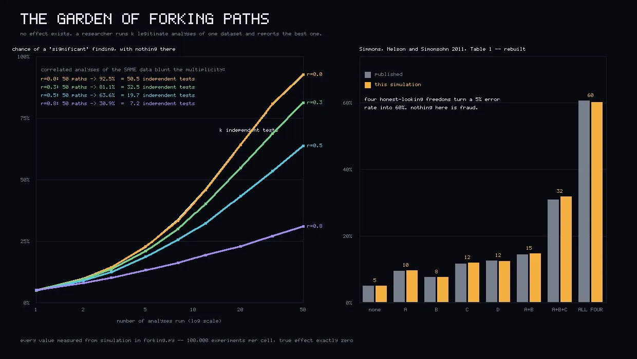
The honest complication is that those fifty analyses are not independent. They are fifty views of the same data, so they rise and fall together, and the multiplicity is blunted. I measured the discount. At a correlation of 0.5, which is a mild assumption for analyses of one dataset, fifty paths buy the error rate of 19.7 independent tests, and the false-positive rate drops from 92.5% to 63.6%. At 0.8 it is worth 7.2 tests and 30.9%.

That blunting is real and it is nowhere near enough. Even the most redundant garden I tested turns a 5% error rate into 31%.

The right panel is a rebuild of the paper that named this problem. In 2011 Simmons, Nelson and Simonsohn took four ordinary researcher freedoms, two outcome measures, adding observations after peeking, controlling for gender, three conditions instead of two, and showed they turn a 5% false-positive rate into 60.7%. My simulation lands within 1.0 points of their published number on every row.

Getting there surfaced something better than a match. Their description of the gender freedom, controlling for gender or for an interaction between gender and the independent variable, does not pin down how many analyses that is. Read literally it is three, and gives 10.3% against their published 11.7%. Add one more analysis any researcher would actually run, the condition effect read off the model that already carries the interaction, and it gives 12.0%.

That single unstated choice moves the headline by 3.9 points. The four-analysis reading then predicts the combined row it was not chosen on: 60.2% against their 60.7%.

The paper measuring how much undisclosed flexibility distorts a result has undisclosed flexibility of its own. I do not think that damages it. I think it is the most honest possible demonstration of its own thesis.

Reading a field from the outside

If you cannot see the file drawer, you can still read the published record, and there is a forensic instrument that works on it. Under a true null, p-values are uniform. So of the significant ones, exactly half fall below .025. Any departure from that flat half means something.

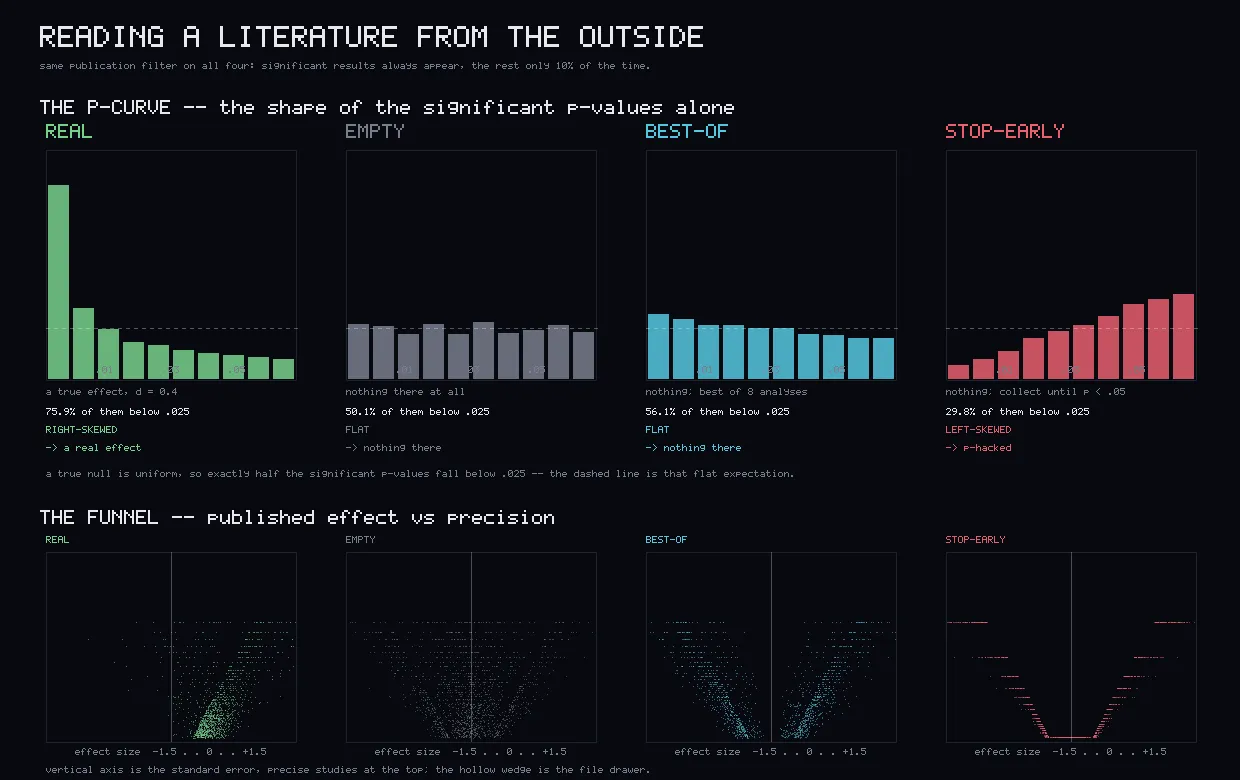
I built four worlds, ran them under one publication filter, and read each only from what got published.

A real effect right-skews the curve hard: 75.9% of its significant p-values sit below .025. An empty, honest field reads 50.1%, which is flat, which is the truth. A field that collects data until it crosses .05 piles its p-values just under the line and reads 29.8%, left-skewed, caught cleanly as hacked.

Three worlds, three correct verdicts, from the published record alone. That is a genuinely good instrument.

The blind spot

Then the fourth world, which I got wrong before I ran it.

I had written into my plan, as settled background, that p-hacking flattens or left-skews the p-curve. That is true of one hacking style. It is false of the most common one.

If a lab runs eight analyses and reports the best, the reported p-value is the minimum of eight. A minimum is pushed down, toward zero, in exactly the same direction a real effect pushes it. Enough forking paths and an empty literature does not go flat. It goes right-skewed, which reads as evidential value.

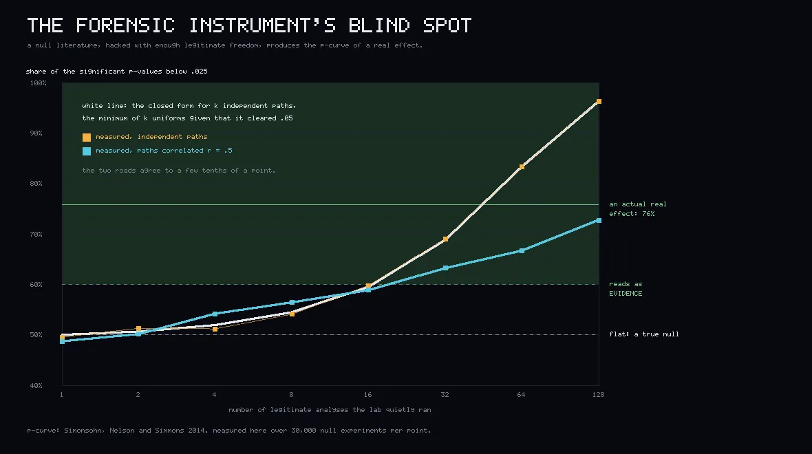
The crossover is computable rather than just observable. For k independent paths, conditional on significance, the share below .025 is

[1 - (1 - a/2)^k] / [1 - (1 - a)^k]

and the simulation matches that closed form to a few tenths of a point from one path to 128. Correlated paths lag behind by exactly the effective-path discount measured earlier.

So here is a field where nothing whatsoever is true. Each lab runs 32 legitimate analyses and, like any field with a predicted direction, believes the ones that came out the expected way.

That literature reports an average effect of d = +0.54. Its p-curve is right-skewed at 65.0%. Its funnel leans, with an Egger test statistic of +50.9, which is the standard signature of publication bias sitting on top of a real finding.

Every instrument agrees it found something. There is nothing there.

The detail that closes the trap is the predicted direction. Undirected hacking leaves a symmetric funnel, and a symmetric funnel is a real tell that something is wrong. A field that knows which way its effect should point erases that symmetry for free, without anyone intending to.

The bias detector is biased

Egger’s test is the standard instrument for detecting publication bias. I ran it on a control literature with no publication filter at all, where it should read zero.

It read +8.9, a confident false alarm, and the reason is arithmetic rather than anything hidden. Cohen’s d is conventionally paired with a standard error that contains d itself, so a large estimate manufactures its own imprecision and the funnel leans on its own algebra. Removing that term dropped the false alarm to +4.7 but did not clear it, because Cohen’s d is also biased upward in small samples, so small studies genuinely do report bigger effects with nothing concealed. Only the bias-corrected effect size with the design-based standard error came back clean at +1.4.

I want to be plain about how close that came to shipping. My control was supposed to read zero. It read +8.9, I fixed the standard error, it read +4.7, and only the third attempt was honest. If I had run the control once and accepted it, I would have published a biased instrument inside an article about biased instruments.

What the corrections buy

The remedies are less interesting than the diagnosis, and more useful.

On a screen of 100 tests with nothing real in it, uncorrected testing reports at least one false discovery in 99% of screens. Bonferroni holds the chance of any false discovery at 5% and pins power at 20% no matter how much real signal is present. Benjamini-Hochberg makes a weaker promise, holding the false share at 5%, and in exchange its power rises with the density of real signal, from 28% to 63% as the real effects go from 5 of 100 to 50 of 100.

Benjamini-Hochberg’s control survived every positive correlation I tested. What correlation costs is power, not control.

The 36%, predicted instead of cited

The famous number is that 36% of psychology findings replicated in the 2015 Open Science Collaboration. I had been citing it all night. The last program predicts it instead.

Take each published significant finding. Power a replication at 90% for that published effect, which is what replicators actually do. Run it honestly. Count.

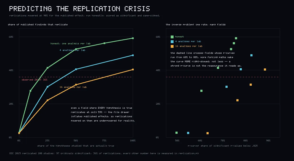
In a field where every hypothesis studied is true and every analysis is honest, only 59% of published findings replicate. Nothing is hidden except the non-significant studies, and that alone is sufficient: the published effect comes out at +0.65 for a true +0.40, so every replication powered on the published number is underpowered for reality. A field where a quarter of hypotheses are true, with total honesty, lands at 41%.

The observed 36% needs no misconduct in it at all.

And then the result I did not expect, which is the right panel. A 36% replication rate does not identify the field. A field where every hypothesis is true and every lab runs 16 analyses replicates at 40.5%. A field where a quarter of hypotheses are true and everyone is scrupulously honest replicates at 41.4%. Same symptom, opposite disease, and opposite fixes.

The p-curve separates them, in the direction opposite to the one I predicted:

all hypotheses true	share of p below .025	replicates
1 analysis per lab	75.7%	58.8%
4 analyses per lab	82.5%	49.0%
16 analyses per lab	88.5%	40.5%

A strongly right-skewed p-curve is not the reassurance it reads as. Only the pair pins a field down. Same skew with a worse replication rate means the hypotheses are empty. Same rate with a flatter curve means the field is honest and underpowered.

Four mistakes, kept

The gender interaction column collapses when a cell happens to be single-sex, and the matrix goes singular. That is not an error to trap: the analysis genuinely cannot be run, so it is reported as p = 1.

I wrote “p-hacking left-skews the p-curve” into the plan as settled and the simulation contradicted it. That correction became the best thing in the folder.

My own control failed twice before it was clean, described above.

And the one that belongs here most. I wrote the conclusion of the replication section before reading the numbers under it, claiming that forking paths drift the p-curve toward flat. The table on the same screen said the opposite. It was caught by reading my own output rather than my own sentence, which is the entire subject of this night, arriving in my own handwriting while I was writing about it.