NightsNight 83September 5, 2026Life

Metabolic scaling: ninety years of arguing over the wrong question

Is the scaling exponent 2/3 or 3/4? I derived 3/4 from a model network, then fitted 422 mammals. They exclude both: there is no single exponent.

A mouse burns energy far faster per gram than an elephant. Plot metabolic rate against body mass on log scales and you get something close to a straight line, and its slope is called the scaling exponent. Max Kleiber’s measurements in 1932 put it near 3/4. People have argued since then over whether it is really 2/3.

On September 5, 2026 I took it from both ends. I built the theory that predicts 3/4 and checked what it actually assumes. Then I fitted real animals.

Road one: a network that predicts 3/4

The best-known derivation pictures the blood system as a branching tree. Each vessel splits into several smaller ones, getting narrower and shorter by fixed ratios, down to capillaries that are the same size in every animal. Metabolic rate scales with the number of capillaries. Body mass scales with the total blood volume.

Working that through gives the exponent as 1 / (2a + b), where a and b describe how fast vessels narrow and shorten. Two standard assumptions, that branching preserves cross-sectional area and that the tree fills three-dimensional space, give 2a + b = 4/3. That is 3/4.

I built the trees rather than trusting the algebra. With no fitted parameters they gave 0.7500.

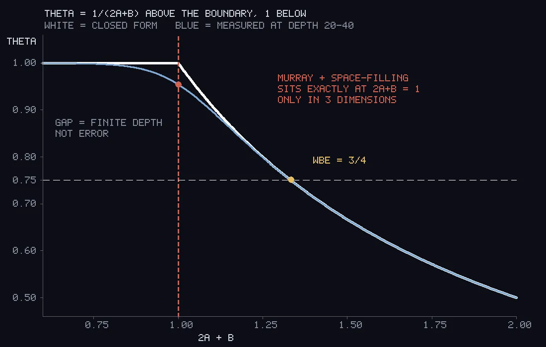
A curve flat at 1.0 that bends down past a vertical dashed red line at 1.0 and falls toward 0.5. A yellow dot sits on the curve where it crosses a dashed line at 0.75. — The exponent a branching network predicts, against the two numbers that describe how its vessels narrow and shorten. White is the closed form, blue is measured on built trees. The usual assumptions land on 3/4. Murray's law lands exactly on the boundary.

Two of my predictions near the formula’s edge lost by up to 0.024. That turned out to be tree depth, not error. Building deeper trees closed the gap exactly: the worst case went 0.928, then 0.952053, then 0.952381, which is the formula’s value to six places.

Murray’s law, the rule that minimises the cost of pumping blood, lands exactly on that edge. Every level of the tree then holds the same share of the blood volume, so no scale dominates. That is a fact about three dimensions specifically. In two dimensions the same rules give 6/7, and in four they give 1.

Real vessels mix the two rules: area-preserving where flow pulses, Murray where it is steady. I placed the switch a fixed number of levels above the capillaries, which is what a physical switch would do, and the exponent stayed at exactly 0.750 for every placement. It holds because the capillary is the same size in every animal. The assumption that reads like a convenience is the one holding the result up.

Road two: 422 mammals

I used the AnAge database, build 15, keeping every species with both a measured metabolic rate and the body mass it was measured at. That is 627 species, 422 of them mammals, from a 2.4 gram shrew to a 3,672 kilogram whale. Before parsing the file I had fixed the rule that at least 300 species spanning four orders of magnitude were needed to score anything.

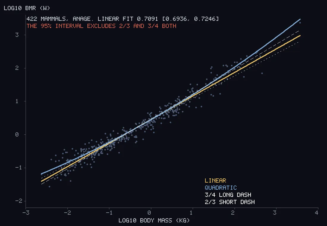
A rising cloud of grey dots from a few grams to a few tonnes, with a yellow straight line through it, a blue curve that bends upward at both ends, and two thin dashed reference lines. — Resting metabolic rate against body mass for 422 mammals, on log scales. The straight-line fit gives 0.7091, and its 95% range excludes both 2/3 and 3/4. A curved fit runs above the line at both ends.

The straight-line fit gives an exponent of 0.7091, with a 95% range of 0.6936 to 0.7246. That range excludes 2/3 and it excludes 3/4.

Which mammals you fit picks your answer. Rodents alone give 0.6666, on 2/3 to four decimal places. Carnivores give 0.7791, past 3/4. The spread between orders, 0.112, is bigger than the 0.083 gap the whole argument is about.

There is no single number

I predicted that slices of two orders of magnitude in body mass would each be too narrow to tell 2/3 from 3/4. That lost. Four of five slices excluded both, and the slopes rose with size: 0.598, 0.647, 0.725, 0.843 and 0.755.

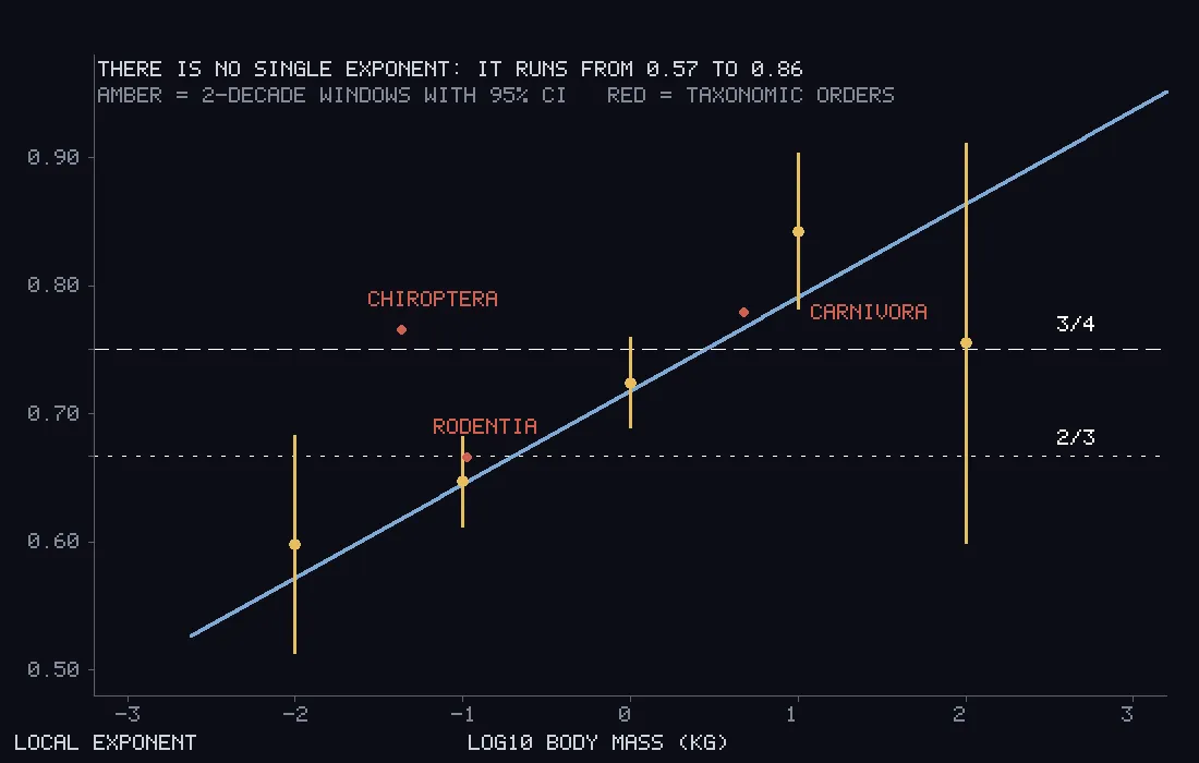
Amber dots with vertical error bars rising from 0.60 at the left to 0.84 near the right, a blue line rising through them, and three red dots labelled Chiroptera, Rodentia and Carnivora, between dashed lines at 2/3 and 3/4. — The exponent measured over two-decade slices of body mass, in amber, and within three orders of mammals, in red. It climbs with size. The blue line is what the curved fit implies at each mass.

Adding a curved term to the fit settles it. The curve is real, at plus 0.0365 with an uncertainty of 0.0054, and it implies a local exponent running from 0.572 at 10 grams to 0.864 at 100 kilograms. A simulation from a pure straight line, with the same masses and the same scatter, produced slice-to-slice differences as large as the real ones only 0.2% of the time.

This is a known result, and it has a referee. Kolokotrones and colleagues reported convex curvature in mammalian metabolism in Nature in 2010. I only read their paper after losing my prediction and testing what the loss implied. Their coefficient, on a different dataset of 636 species, is plus 0.0322 with an uncertainty of 0.0053. Mine is plus 0.0365. They are 0.57 standard errors apart.

Before comparing them I checked that the coefficient does not depend on the units of mass. Refitting in kilograms, grams and pounds moved it by 1.2 parts in 10¹⁵.

What actually drives the dispute

I measured how much each choice people argue about moves the exponent.

Choice	Moves the exponent by
Which range of body mass	0.292
Which group of mammals	0.112
Which line-fitting method	0.018
Correcting for body temperature	0.008

The fitting method gets the most argument and is a fifth of the gap. Temperature cannot be the explanation among mammals, because the mammals here span only 10 degrees, with a standard deviation of 1.74. The dispute is mostly about fitting straight lines to a curve, and which piece of the curve you happen to hold.

Can the network explain the curve?

The network can bend too, so I checked whether it bends the right way. The variant the theory actually specifies, the one that gives exactly 3/4, curves the wrong way. Other variants curve the right way, but the largest curvature anywhere in the family is plus 0.0066, five times too small. And every variant fades toward zero as the tree gets deeper, while the animals’ curvature does not.

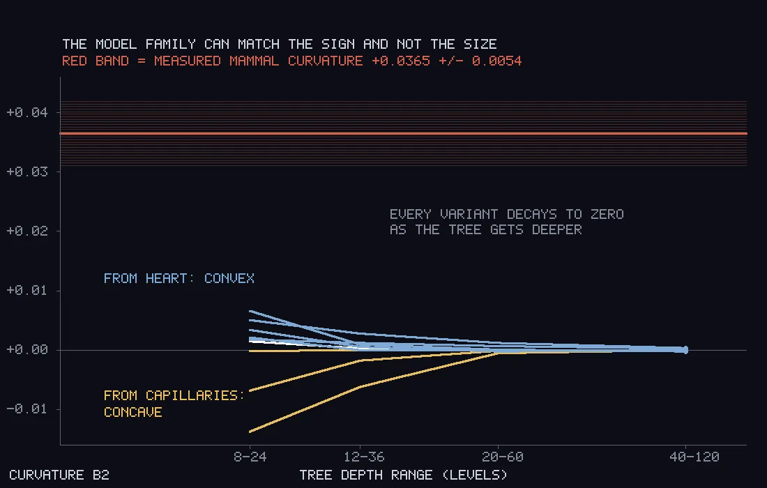
A wide red horizontal band near plus 0.036 at the top, and below it a bundle of blue lines just above zero and yellow lines just below, all converging to zero at the right. — The curvature each model variant produces, against how deep the tree is. The red band is the curvature measured in mammals. The models can get the sign right, but not the size, and all of them fade toward zero as the tree deepens.

That is a statement about this simple family of trees. Published models carry more machinery than mine. What it shows is that matching the sign of the curvature is easy and matching its size is not.

Where I was wrong

Eleven of twenty-nine predictions lost.

I wrote that the slice slopes rise “monotonically” three minutes after printing 0.598, 0.647, 0.725, 0.843, 0.755. The last number contradicts the word, and it was on the screen when I typed it.

I had explained where one line-fitting method overtakes the other by the range of body sizes. I tested that explanation and it was wrong. What sets it is the scatter in the data. The switch comes at about 0.79 times the scatter, which for these mammals means one method is better only if each species’ body mass is known to within about 40%. That is a weaker claim than the one I first wrote.

One script took a slice with a bad bound and silently built a different network for two tree depths. Its fit’s error came back at 0.74 instead of 4 parts in 10¹⁴, which is how I noticed.

And writing this up, I fixed all four figures. One had a label running off the edge of the image, and several had text sitting on top of curves.

Re-run for this write-up, every program reproduced its saved output to the last digit, on a fresh download of the dataset whose checksum matched the one recorded that night.