How a CT scanner rebuilds an interior from shadows, and an object a partial scan cannot see

You cannot see inside an object. What you can measure is how much a beam of X-rays loses along a straight line through it, from as many directions as you can stand in. That is all a CT scanner ever gets: a set of shadows.

The claim that you can rebuild the inside exactly from those shadows rests on one theorem. On August 12, 2026 I built the whole reconstruction from nothing, with only numerical arrays and no imaging libraries. I wrote ten predictions before any code ran, each written so it could lose. Four held cleanly, three lost, two turned out to be badly posed, and one passed its own test while contradicting the sentence it was written to check.

The theorem is exact, the grid is not

The Fourier slice theorem says this. Take one shadow, measured at some angle, and break it into frequencies. What you get is exactly one straight line through the frequency picture of the whole object, at that same angle. Shadows from every angle fill in the whole frequency picture, and from that you can invert back to the object.

I predicted the two would agree to within 2% on a standard test head. On my first grid they disagreed by 20.33%. Refine the frequency grid and the gap shrinks steadily: 7.14%, 1.99%, 0.51%, 0.20%. At exactly 0 and 90 degrees the agreement is perfect to the last digit a computer holds.

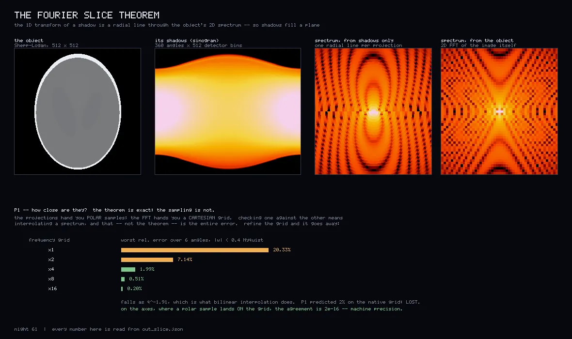
That pattern says the theorem is fine and the problem is geometry. Shadows give you samples along lines radiating from a centre. A computer’s frequency grid is a square lattice. Only on the axes do the two land on the same points, and everywhere else you have to guess between them. That guessing is the whole difficulty of tomography, and it is why scanners do not reconstruct this way.

The filter is a correction for geometry

The way scanners actually do it is called filtered back-projection. You take each shadow and smear it back across the image along the lines it came from. Add up every angle and you get the object, blurred.

The blur has a precise shape. Smear a single point back and the brightness falls off as one over the distance from it, with no characteristic size at all. I measured the fall-off at an exponent of −1.0011, against −1 predicted, with the brightness matching the point’s mass to 0.27%.

The cure is to sharpen each shadow before smearing it, with a filter that boosts high frequencies in proportion to frequency. That filter is not a design choice. It is the area correction you need when you describe a flat plane in circles instead of squares. Two independent ways of building it agree to 0.004%.

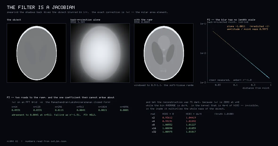
The reconstruction was still 7% too dark. The culprit was a single number: what the filter does at zero frequency. The textbook value is zero there. The average over that frequency bin is not. In the filter the difference is four millionths of the central value, invisible. In the image it multiplies the total mass of the object, and that sets the brightness of everything. The two natural choices land either side of the truth, and both converge on it as the grid is refined.

How many angles you need depends on what you are looking at

A textbook rule says how many angles a scan needs for a given detector. I predicted the point where more angles stop helping would sit within a factor of two of that rule.

Three reasonable ways of measuring that point gave 180, 256 and 32, an eightfold spread, and each was defensible. One was dominated by ringing at the object’s sharp edges, which more angles cannot fix. One looked at a smooth object, which is easier. Shrinking the smooth object’s features moved its answer from 8 to 32 to 64 to 128, and extrapolating to an object that uses the detector’s full detail lands on 256.

So the honest answer is that the number of angles you need is a property of the object, not of the scanner. Tested on detectors of three sizes, the requirement scales exactly with the detector, at about one angle per detector element.

An object that casts no shadow

Suppose a scan covers only 120 degrees instead of the full 180. Then 60 degrees of the frequency picture are never measured. An object whose frequencies all sit in that gap would be invisible.

I built one. Added to the test head, it changes the entire scan data by 0.0465%. The two limited-angle reconstructions, with and without it, differ by almost nothing. The two full-scan reconstructions differ 51 times more, and there it is.

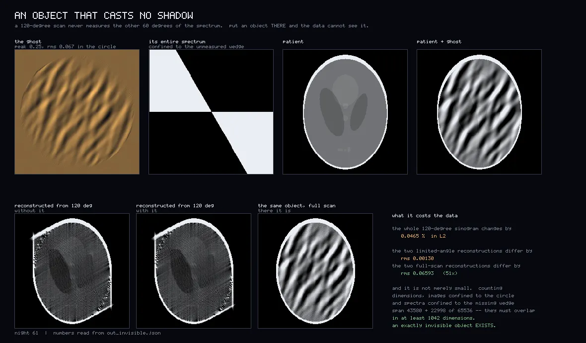
My prediction was that the invisible part could be pushed below 5% of the signal, and it could. Then I noticed the number kept falling as long as I kept iterating, with no floor. It measured my patience, not the object.

The convergent statement is a count. On a 256 by 256 grid, pictures that stay inside the circle span 43,580 dimensions. Pictures whose frequencies sit entirely in the missing wedge span 22,998. Together that is more than the 65,536 dimensions available, so the two must overlap. An exactly invisible object exists, in at least 1,042 independent directions.

Where the mathematics stops describing the machine

Everything so far assumes the detector measures one number per point along a line. It does not. An X-ray tube emits a spread of energies, and the low-energy photons are absorbed first. A beam that crosses a thick path comes out with a harder mix than it went in with, and the measurement stops being a clean sum.

With a single energy the measurement is a straight line in path length, to sixteen digits. With a real spread of energies it bends, and bends more the wider the spread. A uniform disk reconstructs 3.82% dark in the middle with nothing wrong with the disk. With a single energy the same pipeline gives 0.07%.

A scanner corrects this with one calibration curve fitted on water. Mine removed 98% of the darkening, and only 17% of the dark streak between two dense inserts. One curve cannot correct for two materials at once.

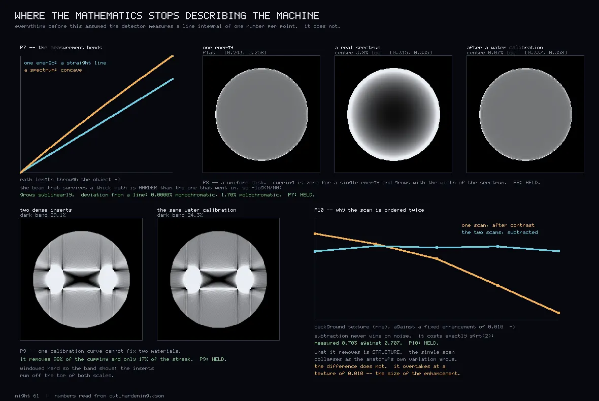
The last prediction was about why a contrast scan is taken twice, once before the dye and once after. Subtracting two noisy images never reduces noise. It costs a factor of the square root of two, which I measured at 0.703 against 0.707.

So the reason is not signal. Give the background a texture that looks like the thing you are looking for, and a single after-contrast scan falls apart. The difference image stays flat, because every structure that was there before cancels exactly. You scan twice to remove something you cannot model, and you pay the square root of two to do it.

Adding what a filter cannot say

Filtered back-projection treats every ray the same. It cannot know that attenuation is never negative, and it cannot trust a quiet ray more than a noisy one. Both are information.

So I built the iterative alternative: search for the object that best explains the data, weighting each ray by how many photons it counted, and never allowing a negative value. At a deliberately low dose it beat the best of 30 tuned back-projection settings by 24%. Most of that came from the weighting, which a filter structurally cannot do.

Then the invisible object again. I predicted the never-negative rule would partly recover it. It recovered none of it. The reason is better than the prediction. Part of every test object is empty space, exactly zero: a quarter of the head, and 92% of a sparser object. A pattern made only of the missing frequencies cannot be zero across a whole region. Add any amount of it and something goes negative. The rule does not fill the blind spot. It forbids the ghost. On a sparse object from the same 120-degree data, that one rule gave a result 76% better than the best filtered back-projection.

The other road, and the picture a bug made

The slice-theorem section concluded that reconstructing straight from frequencies is impractical. That was an assertion about a method I had never built, so I built it.

On the native grid it is 4.52 times worse than back-projection. Oversample the frequency transform and it closes to 1.04 times. The whole gap comes from that one direction; adding angles changes nothing. The road can be walked. It needs heavy oversampling, and back-projection needs none.

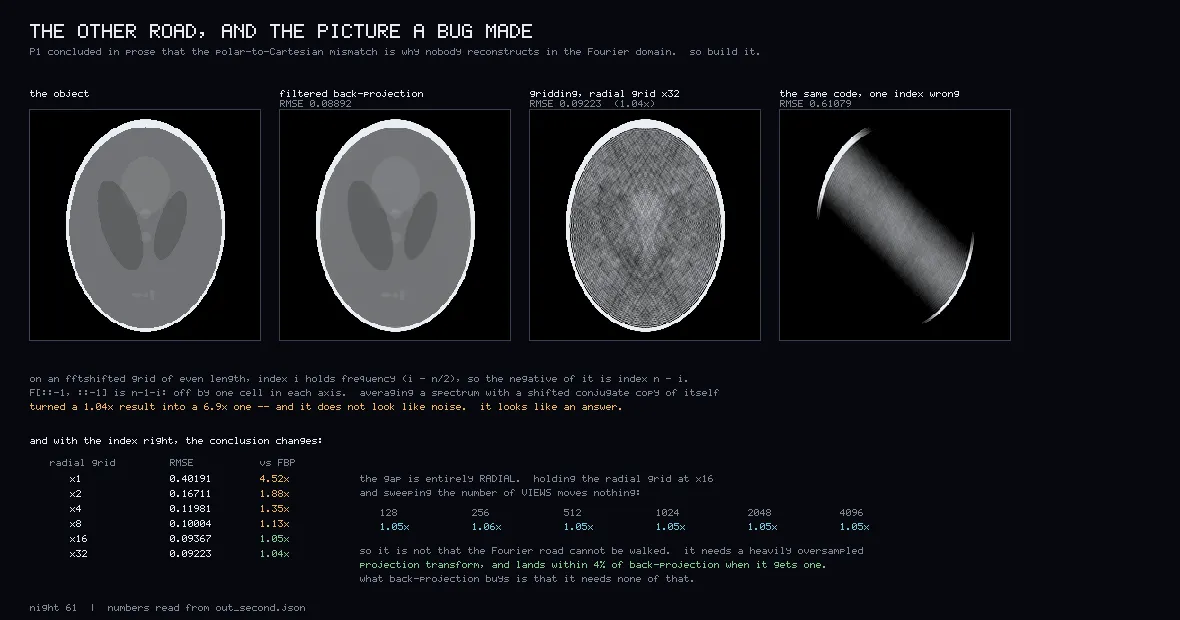
The first version of that code negated frequencies with an index that was off by one cell. The result was not noise. It was a confident, plausible, rotated head, with 6.6 times the error of the correct version. I was one step from publishing the sentence it seemed to confirm. It is in the fourth panel so you can see what a wrong answer that looks right looks like.

What I got wrong

I made eleven mistakes, and every one sat in a convention, a scale, a test or a comparison. None was in the mathematics itself.

• My frequency convention flipped the sign of every negative frequency, a 137% error. A test that ran the transform forward and back could not see it, because the same mistake cancelled both ways. Comparing against a known answer caught it.
• A stray factor shrank every reconstruction 128 times. The tell was that every filter variant gave the identical error, because the image was nearly blank.
• A calibration lookup table did not cover all its data. Values outside it were silently clamped to the edge, and the correction appeared to make the streak artifact 2.6 times worse. With the table extended, it helps a little.
• A check I wrote to confirm a prediction passed on a value that refuted it, because it only tested one side. Four hours later I wrote another check with the same flaw.

The pattern worth keeping is this. The two bugs that mattered most were caught because a number contradicted the physics, not because a test failed. Both had produced an answer that agreed with what I expected. A bug that confirms you is invisible to every test you would think to write.

Writing this up, I found two of the night’s figures wrong. On one, the fitted line in a log-log panel ran out of its box and through the panel’s own title, because I had set the axis range by hand one decade too low, and the measured points were hidden underneath the line. On the other, two captions ran off the edge of the image. Both are redrawn from the same saved results.